Using Avogadro2 with Gaussian and ORCA on Roihu
Avogadro2 is a program for building, visualizing and analyzing molecules, with input generators for several quantum chemistry programs. On Roihu it runs in the Desktop app of the web interface, so you can build a molecule, create an input file, and open the result in one place. In this tutorial you build ethanol, optimize it, and run a geometry optimization with Gaussian (B3LYP) or ORCA (r2SCAN-3c).
For all options, see the Avogadro2, Gaussian and ORCA pages.
1. Start Avogadro2
- In the Roihu web interface, select Apps → Desktop.
- Select your Project and the Partition
interactive, set Memory (GiB) to 4, and click Launch. - In My Interactive Sessions, click Launch Desktop when the session is Running.
- On the desktop, double-click the Avogadro 2 icon. If a Version Update window appears, select Ignore.
See the Desktop page for more.
2. Build ethanol
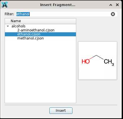
Select Build → Insert → Molecule..., type ethanol in the Filter field, select ethanol.cjson in the alcohols category, and click Insert.
To draw a molecule instead, see Building a structure.
3. Optimize with a force field
Select Extensions → Open Babel → Optimize Geometry. This gives a reasonable start geometry. To change the force field, use Extensions → Open Babel → Configure Force Field....
4. Create the input file
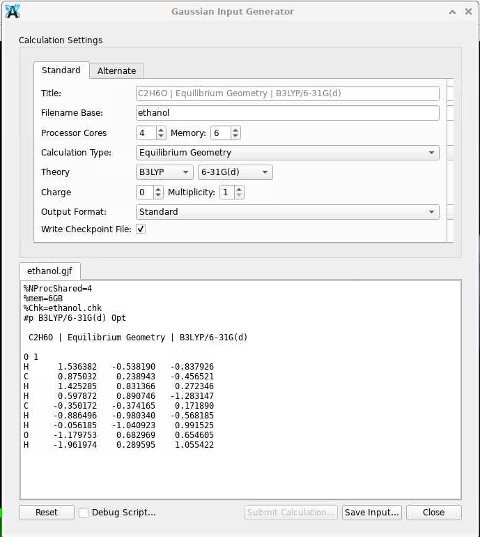
Open the generator from the Input menu. Set the processor cores to 4 and the total memory to 6 GB.
Select Input → Gaussian....
| Setting | Value |
|---|---|
| Filename Base | ethanol |
| Processor Cores | 4 |
| Memory | 6 GB |
| Calculation Type | Equilibrium Geometry |
| Theory | B3LYP, 6-31G(d) |
| Charge / Multiplicity | 0 / 1 |
| Write Checkpoint File | on |
The preview shows %NProcShared=4, %mem=6GB, %Chk=ethanol.chk and the route line #p B3LYP/6-31G(d) Opt.
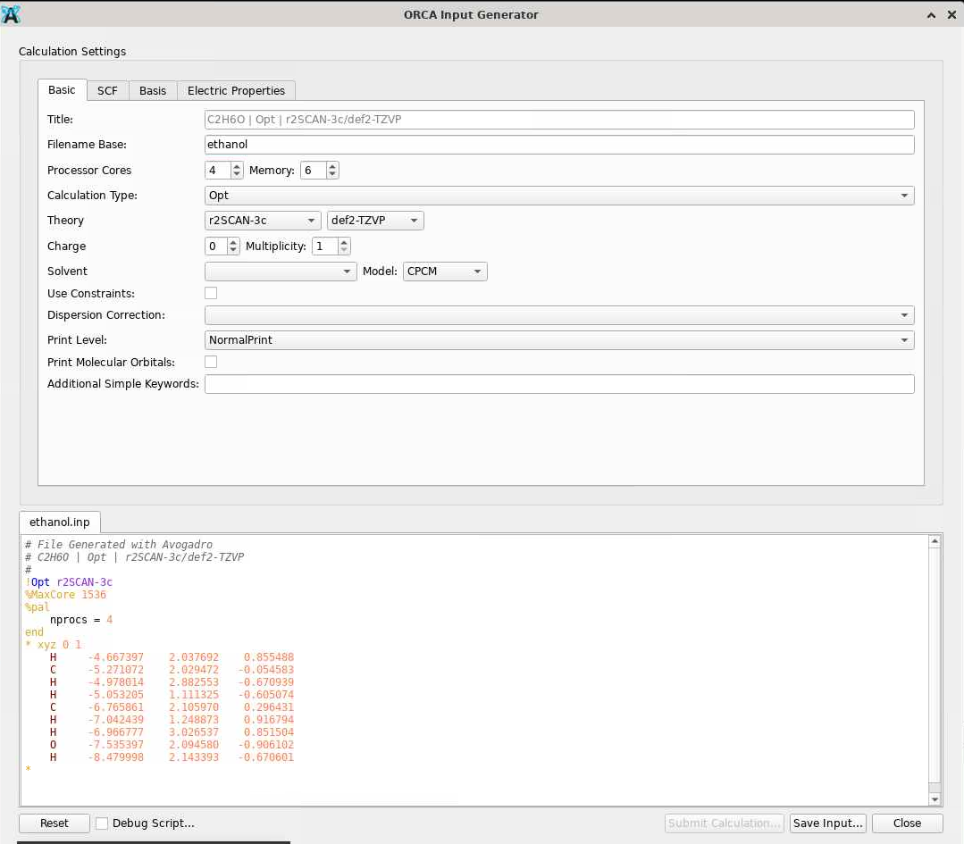
Select Input → ORCA....
On the Basic tab:
| Setting | Value |
|---|---|
| Filename Base | ethanol |
| Processor Cores | 4 |
| Memory | 6 GB |
| Calculation Type | Opt |
| Theory | r2SCAN-3c (default) |
| Charge / Multiplicity | 0 / 1 |
| Print Molecular Orbitals | off |
r2SCAN-3c is a composite method with its own basis set, so no basis set is given in the keyword line. The input has nprocs = 4 in the %pal block and %MaxCore 1536 (MB per process).
Click Save Input.... Use a separate directory for each calculation. In the file dialog, type /scratch/<project> in the File name field and press Enter to go to the project directory. Then click Create New Folder (the folder icon with a plus sign at the top right), type ethanol_opt as the name of the new folder, press Enter, and double-click the folder to open it. Type the file name ethanol.com for Gaussian (the dialog proposes ethanol.gjf, but subg16 needs the extension .com) or ethanol.inp for ORCA, and click Save. The generators only write the input file. The program must be available on Roihu.
5. Run the calculation
Run the calculation as a batch job. Submit it from the Roihu CPU login node (roihu-cpu.csc.fi). The login nodes share the same files, so the input file that you saved in the Desktop session is also there.
Keep the Desktop session open and open a second terminal on the CPU login node, in one of two ways:
- In the Roihu web interface, start Login node shell (Roihu-CPU) from the pinned apps in a new browser tab.
- From your own computer, connect with SSH:
ssh <username>@roihu-cpu.csc.fi. See Connecting.
The arguments are the run time, the job name (the input file ethanol.com without the extension), and the billing project. The number of cores and the memory are read from %NProcShared and %mem in the input file.
ORCA is not installed centrally at CSC. Install a private copy first, see the ORCA page.
Create job.sh in the same directory as ethanol.inp:
#!/bin/bash
#SBATCH --partition=small
#SBATCH --nodes=1
#SBATCH --ntasks-per-node=4       # same as %pal nprocs
#SBATCH --mem-per-cpu=1536        # MB, same as %MaxCore
#SBATCH --account=<project>
#SBATCH --time=00:30:00

export ORCADIR=/projappl/<project>/<user>/orca/<orca-directory>
module purge
module load orca/6.1.1

${ORCADIR}/orca ethanol.inp > ethanol.out
The calculation takes less than a minute. The time in the queue can be longer.
6. Check the result
Check the job with:
The job is finished when it is no longer in the list. Then check the end of the output:
Both lines should be printed.
7. View the optimized structure
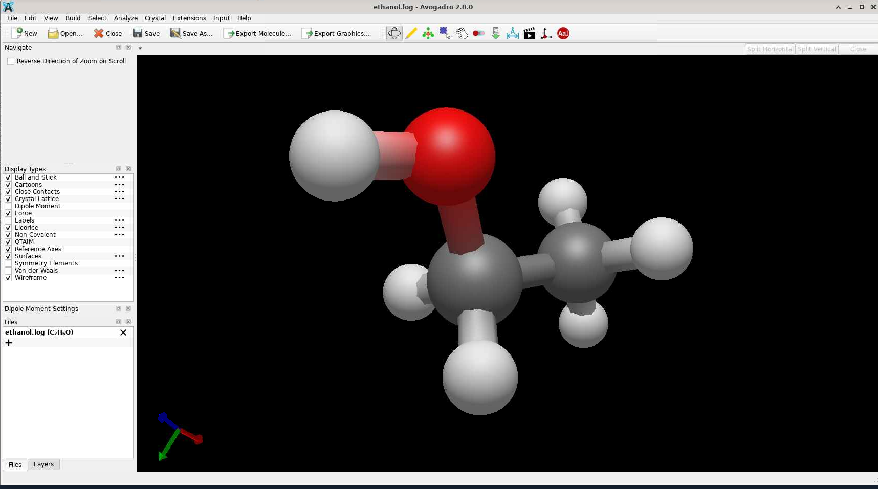
In Avogadro2, select File → Open and open the output file: ethanol.log (Gaussian) or ethanol.out (ORCA). The file dialog may open in another directory, so type the full path of the file in the File name field. If Avogadro2 asks to save the changes, select Discard. The input file is already saved.
The window shows the optimized structure. The Player has one frame. The energy of each step is in the log:
The file holds all optimization steps. Click the clapperboard icon in the toolbar to open the Player, and use the slider or the < and > buttons to step through the geometries. The file opens at the first frame, and the last frame is the optimized structure. Compare it with the first frame, for example the C–O bond length.
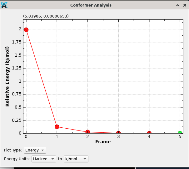
To see the energy of each step, select Analyze → Plot Conformer Data... and the plot type Energy. The plot shows the energy relative to the lowest-energy step (the last one) against the frame number.
8. Frequency calculation
A frequency calculation confirms that the optimized structure is a minimum. It must use the optimized structure and the same model chemistry (method and basis set) as the optimization:
- In Avogadro2, open the output file of the optimization (see step 7). For ORCA, select the last frame in the Player. The window now holds the optimized structure. Do not run the force-field optimization again.
- Open the input generator (it starts with default values) and use the settings of step 4, except Filename Base
ethanol_freq, Calculation TypeFrequencies(Gaussian) orFreq(ORCA), and Print Molecular Orbitals on (ORCA, see step 9). The preview showsFreqin the keyword line. - Click Save Input... and save the file in the same directory as
ethanol_freq.com(Gaussian) orethanol_freq.inp(ORCA).
Submit the job as in step 5, with the new name:
When the job has finished, open the result in Avogadro2:
Select Analyze → Vibrational Modes....
A minimum has no imaginary frequencies. An imaginary frequency is shown as a negative number. ORCA also lists six zero frequencies first (translations and rotations). One imaginary frequency means a transition state, or a structure that needs more optimization. Select a mode to animate it, or select Analyze → Plot Spectra... for the IR spectrum.
To optimize and calculate the frequencies in one job, add Freq to the job line of the input of step 4 (#p B3LYP/6-31G(d) Opt Freq for Gaussian, !Opt r2SCAN-3c Freq for ORCA).
9. Molecular orbitals
The frequency calculation also gives the orbitals at the optimized geometry.
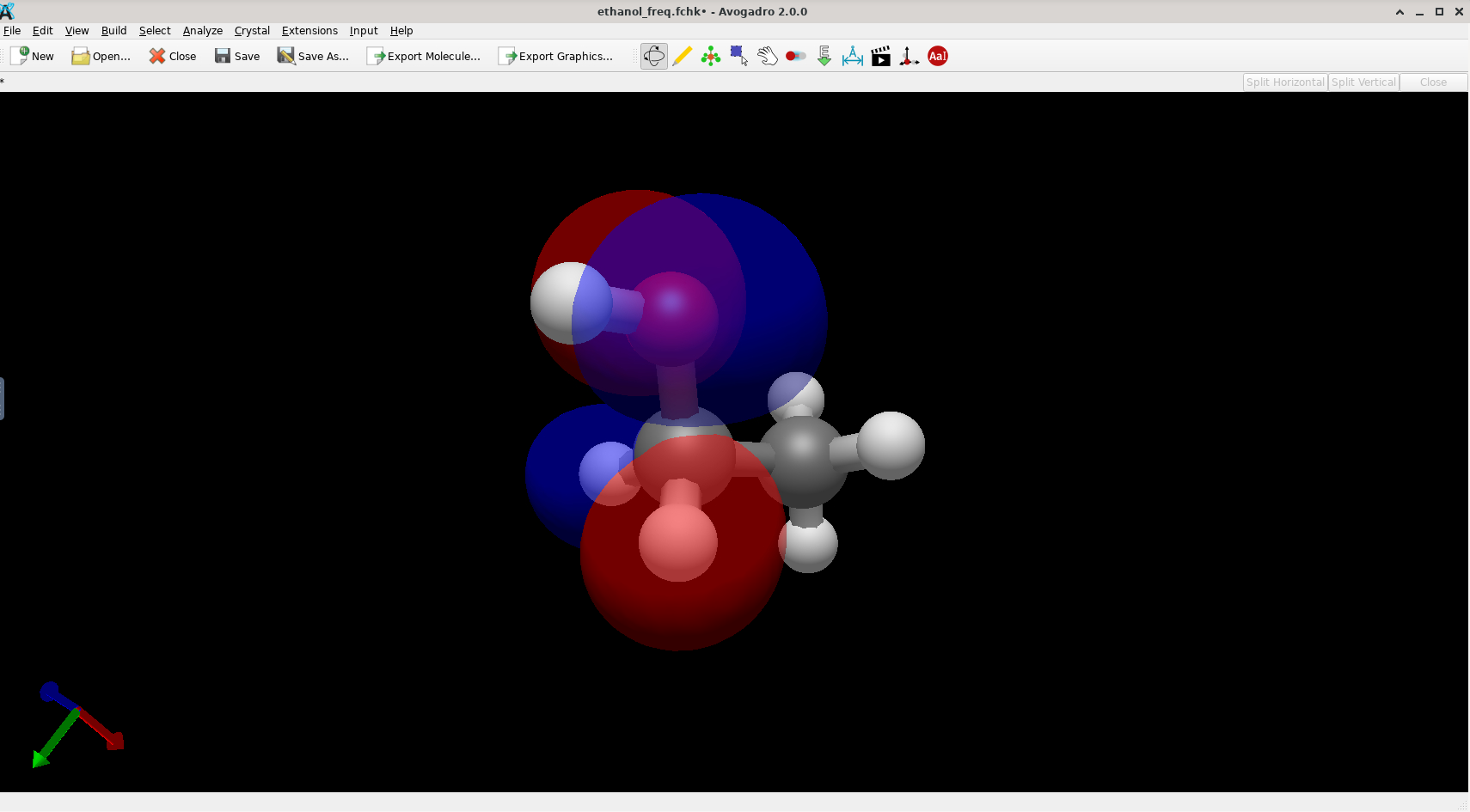
Open ethanol_freq.fchk from step 8 in Avogadro2.
The option Print Molecular Orbitals adds PrintMOs PrintBasis to the input, so the orbitals are in ethanol_freq.out. Open it in Avogadro2.
Select Analyze → Molecular Orbitals.... The window lists the orbitals with their energies and occupations. The list starts with the highest orbital, so scroll down to HOMO and LUMO. Select HOMO or LUMO, set the Quality, and click Render.
Hints
Start with a cheap method and refine the result step by step. This saves resources while the structure is still far from the minimum:
- Optimize with a force field in Avogadro2 (step 3).
- Optimize with a small basis set or a composite method, as in this tutorial.
- Calculate the final energy with a larger basis set or a more accurate method at the optimized geometry.
Use the output of each step as the start structure of the next step (open it in Avogadro2, see step 8), and check that each calculation finished normally before you continue.
See the Gaussian and ORCA pages for more.